
[pytorch] pretrained model의 활용과 fine tuning 하기
업데이트:
개요

이번 포스팅은 pytorch에서 transfer learning을 적용하는 방법에 관한 내용이다.
transfer learning은 학습 데이터셋이 적거나 컴퓨팅 자원이 적을 때, 이미 학습되어진 model parameter를 이용해서 나의 task에 맞도록 조정(fine-tuning)하는 방법이다.
Task나 dataset에 따라, 기존 layer에서 어디까지 고정(freeze)하고 어디부터 다시 train 시킬지(fine-tuning)가 중요하다. 이번 포스팅에서 경험적으로 fine tuning 하는 과정을 배워보자.
Data Loading
이전 tutorial과 마찬가지로 CIFAR10 데이터 셋을 이용한다.
# pytorch
import torch
import torchvision
from torchvision import transforms, datasets, models
from torchsummary import summary

import torch.nn as nn
import torch.nn.functional as F
import torch.optim as optim

device = 'cuda' if torch.cuda.is_available() else 'cpu'

# other
import numpy as np
import matplotlib.pyplot as plt
import copy
import time
batch_size=200
transform = transforms.Compose([
            transforms.ToTensor(),
            transforms.Normalize((0.5,0.5,0.5),(0.5,0.5,0.5))
])
trainset = datasets.CIFAR10(root='dataset/',train=True,
                                        download=True,transform=transform)
trainloader = torch.utils.data.DataLoader(trainset, batch_size=batch_size,
                                          shuffle=True, num_workers=2)
testset = datasets.CIFAR10(root='dataset/',train=False,
                                       download=True,transform=transform)
testloader = torch.utils.data.DataLoader(testset, batch_size=batch_size,
                                          shuffle=False, num_workers=2)
classes = ('plane', 'car', 'bird', 'cat', 'deer',
           'dog', 'frog', 'horse', 'ship', 'truck')
- 샘플 데이터 시각화
test = iter(trainloader)
images, labels = next(test)

def imshow(img):
    img = img / 2 + 0.5     # unnormalize
    npimg = img.numpy()
    plt.imshow(np.transpose(npimg, (1, 2, 0)))
    plt.show()

# imshow(torchvision.utils.make_grid(images))
imshow(images[0])
print(classes[labels[0]])
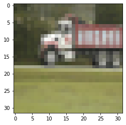
truck
Modeling
Pretrained model
pytorch의 torchvision.models에서는 ImageNet 기반의 pretrained model들을 제공하고 있다.
예를들면, 이전에 공부했던 ResNet, AlexNet, VGG, GoogLeNet 등이 있다.
여기서는 ResNet18을 사용해보려고 한다. 필요한 두가지 작업은 아래와 같다.
- 기존 layer의 weight를 고정(freeze)
- 마지막 fully-connected layer를 task(class)에 맞도록 변경(fine-tuning)
이렇게 하면 기존 weight들은 그대로 사용하고, 마지막 fc layer만 튜닝해서 최소한의 학습을 통해 모델링을 할 수 있다.
아래와 같이 pretrained=True인자를 넣어주면, 기본적으로 ImageNet에 학습된 weight을 불러와 주지만, 최근에는 ImageNet version에 따라 weight을 불러와서 입력해주는 것을 권장하고 있다.
자세한 내용은 공식 document를 참고하자.
resnet_pt = models.resnet18(pretrained=True)
# freezing
for param in resnet_pt.parameters():
    param.requires_grad = False

# fc layer 수정
fc_in_features = resnet_pt.fc.in_features
resnet_pt.fc = nn.Linear(fc_in_features, len(classes))
resnet_pt = resnet_pt.to(device)
torchsummary를 통해 model을 확인해보면, parameter들에 대한 정보를 알 수 있다.
- 전체 parameter 수(
Total params): 11,181,642 - 학습가능한 parameter 수(
Trainable params): 5,130 - freeze된 parameter 수(
Non-trainable params): 11,176,512
마지막 Avgpooling layer를 통해 output size는 512이고, 이걸 받아서 fc는 10을 내보내므로 학습가능한(trainable) 파라미터 수는 512 x 10 + 10(bias)=5,130이 되는 것이다.
summary(resnet_pt, (3,32,32))
----------------------------------------------------------------
        Layer (type)               Output Shape         Param #
================================================================
            Conv2d-1           [-1, 64, 16, 16]           9,408
       BatchNorm2d-2           [-1, 64, 16, 16]             128
              ReLU-3           [-1, 64, 16, 16]               0
         MaxPool2d-4             [-1, 64, 8, 8]               0
            Conv2d-5             [-1, 64, 8, 8]          36,864
       BatchNorm2d-6             [-1, 64, 8, 8]             128
              ReLU-7             [-1, 64, 8, 8]               0
            Conv2d-8             [-1, 64, 8, 8]          36,864
       BatchNorm2d-9             [-1, 64, 8, 8]             128
             ReLU-10             [-1, 64, 8, 8]               0
       BasicBlock-11             [-1, 64, 8, 8]               0
           Conv2d-12             [-1, 64, 8, 8]          36,864
      BatchNorm2d-13             [-1, 64, 8, 8]             128
             ReLU-14             [-1, 64, 8, 8]               0
           Conv2d-15             [-1, 64, 8, 8]          36,864
      BatchNorm2d-16             [-1, 64, 8, 8]             128
             ReLU-17             [-1, 64, 8, 8]               0
       BasicBlock-18             [-1, 64, 8, 8]               0
           Conv2d-19            [-1, 128, 4, 4]          73,728
      BatchNorm2d-20            [-1, 128, 4, 4]             256
             ReLU-21            [-1, 128, 4, 4]               0
           Conv2d-22            [-1, 128, 4, 4]         147,456
      BatchNorm2d-23            [-1, 128, 4, 4]             256
           Conv2d-24            [-1, 128, 4, 4]           8,192
      BatchNorm2d-25            [-1, 128, 4, 4]             256
             ReLU-26            [-1, 128, 4, 4]               0
       BasicBlock-27            [-1, 128, 4, 4]               0
           Conv2d-28            [-1, 128, 4, 4]         147,456
      BatchNorm2d-29            [-1, 128, 4, 4]             256
             ReLU-30            [-1, 128, 4, 4]               0
           Conv2d-31            [-1, 128, 4, 4]         147,456
      BatchNorm2d-32            [-1, 128, 4, 4]             256
             ReLU-33            [-1, 128, 4, 4]               0
       BasicBlock-34            [-1, 128, 4, 4]               0
           Conv2d-35            [-1, 256, 2, 2]         294,912
      BatchNorm2d-36            [-1, 256, 2, 2]             512
             ReLU-37            [-1, 256, 2, 2]               0
           Conv2d-38            [-1, 256, 2, 2]         589,824
      BatchNorm2d-39            [-1, 256, 2, 2]             512
           Conv2d-40            [-1, 256, 2, 2]          32,768
      BatchNorm2d-41            [-1, 256, 2, 2]             512
             ReLU-42            [-1, 256, 2, 2]               0
       BasicBlock-43            [-1, 256, 2, 2]               0
           Conv2d-44            [-1, 256, 2, 2]         589,824
      BatchNorm2d-45            [-1, 256, 2, 2]             512
             ReLU-46            [-1, 256, 2, 2]               0
           Conv2d-47            [-1, 256, 2, 2]         589,824
      BatchNorm2d-48            [-1, 256, 2, 2]             512
             ReLU-49            [-1, 256, 2, 2]               0
       BasicBlock-50            [-1, 256, 2, 2]               0
           Conv2d-51            [-1, 512, 1, 1]       1,179,648
      BatchNorm2d-52            [-1, 512, 1, 1]           1,024
             ReLU-53            [-1, 512, 1, 1]               0
           Conv2d-54            [-1, 512, 1, 1]       2,359,296
      BatchNorm2d-55            [-1, 512, 1, 1]           1,024
           Conv2d-56            [-1, 512, 1, 1]         131,072
      BatchNorm2d-57            [-1, 512, 1, 1]           1,024
             ReLU-58            [-1, 512, 1, 1]               0
       BasicBlock-59            [-1, 512, 1, 1]               0
           Conv2d-60            [-1, 512, 1, 1]       2,359,296
      BatchNorm2d-61            [-1, 512, 1, 1]           1,024
             ReLU-62            [-1, 512, 1, 1]               0
           Conv2d-63            [-1, 512, 1, 1]       2,359,296
      BatchNorm2d-64            [-1, 512, 1, 1]           1,024
             ReLU-65            [-1, 512, 1, 1]               0
       BasicBlock-66            [-1, 512, 1, 1]               0
AdaptiveAvgPool2d-67            [-1, 512, 1, 1]               0
           Linear-68                   [-1, 10]           5,130
================================================================
Total params: 11,181,642
Trainable params: 5,130
Non-trainable params: 11,176,512
----------------------------------------------------------------
Input size (MB): 0.01
Forward/backward pass size (MB): 1.29
Params size (MB): 42.65
Estimated Total Size (MB): 43.95
----------------------------------------------------------------
Training
이제 learning process에 맞게 간단한 code를 구현하고 돌려보도록 하자.
- loss, optimizer, lr scheduler를 정의
criterion = nn.CrossEntropyLoss()
optimizer = optim.SGD(resnet_pt.parameters(), lr=0.001,
                      momentum=0.9)
scheduler = torch.optim.lr_scheduler.CosineAnnealingLR(optimizer, T_max=200)
- Train과 Test를 위한 function 정의
# Training
def train(epoch, model, criterion, optimizer):
    model.train()
    train_loss = 0
    correct = 0
    total = 0
    for batch_idx, (inputs, labels) in enumerate(trainloader):
        inputs, labels = inputs.to(device), labels.to(device)
        optimizer.zero_grad()
        outputs = model(inputs)
        loss = criterion(outputs, labels)
        loss.backward()
        optimizer.step()

        train_loss += loss.item()*inputs.size(0)
        _, predicted = outputs.max(1)
        total += labels.size(0)
        correct += predicted.eq(labels).sum().item()

    epoch_loss = train_loss/total
    epoch_acc = correct/total*100
    print("Train | Loss:%.4f Acc: %.2f%% (%s/%s)"
        % (epoch_loss, epoch_acc, correct, total))
    return epoch_loss, epoch_acc

def test(epoch, model, criterion, optimizer):
    model.eval()
    test_loss = 0
    correct = 0
    total = 0
    with torch.no_grad():
        for batch_idx, (inputs, labels) in enumerate(testloader):
            inputs, labels = inputs.to(device), labels.to(device)
            outputs = model(inputs)
            loss = criterion(outputs, labels)

            test_loss += loss.item()*inputs.size(0)
            _, predicted = outputs.max(1)
            total += labels.size(0)
            correct += predicted.eq(labels).sum().item()

        epoch_loss = test_loss/total
        epoch_acc = correct/total*100
        print("Test | Loss:%.4f Acc: %.2f%% (%s/%s)"
            % (epoch_loss, epoch_acc, correct, total))
    return epoch_loss, epoch_acc
- Main code에서 learning 시작
start_time = time.time()
best_acc = 0
epoch_length = 100
save_loss = {"train":[],
             "test":[]}
save_acc = {"train":[],
             "test":[]}
for epoch in range(epoch_length):
    print("Epoch %s" % epoch)
    train_loss, train_acc = train(epoch, resnet_pt, criterion, optimizer)
    save_loss['train'].append(train_loss)
    save_acc['train'].append(train_acc)

    test_loss, test_acc = test(epoch, resnet_pt, criterion, optimizer)
    save_loss['test'].append(test_loss)
    save_acc['test'].append(test_acc)

    scheduler.step()

    # Save model
    if test_acc > best_acc:
        best_acc = test_acc
        best_model_wts = copy.deepcopy(resnet_pt.state_dict())
    resnet_pt.load_state_dict(best_model_wts)

learning_time = time.time() - start_time
print(f'**Learning time: {learning_time // 60:.0f}m {learning_time % 60:.0f}s')
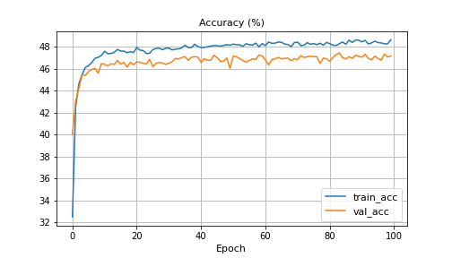
이미 만들어진 feature만을 가지고 fc만 tuning했을때는 약 48% 정도가 나온다.
초반 20 epoch 정도에서 달성되고 이후로는 더디게 증가하는데, fc layer만 fine tuning 해야하는 한계로 보인다.
그래도 고정된 weight만 가지고도 50%정도의 정확도가 나오는 것은 긍정적(?)인 것 같다.
Fine tuning
몇 가지 다른 방법을 시도해보자.
pretrained model 전체 layer 재학습
위 코드를 기반으로 아래와 같이 전체 layer에 대해 freeze했던 것을 제외하고, 다시 학습을 진행한다.
이렇게 진행할 경우 ResNet18로 학습을 하되, weight의 random initialize 대신 학습된 weight을 초기값으로 학습을 시작하게 된다.
resnet_pt = models.resnet50(pretrained=True)
# for param in resnet_pt.parameters():
#     param.requires_grad = False
fc_in_features = resnet_pt.fc.in_features

resnet_pt.fc = nn.Linear(fc_in_features, len(classes))
resnet_pt = resnet_pt.to(device)
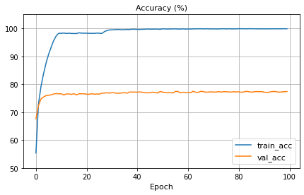
결과적으로 정확도는 초반부터 급격하게 증가했으나, training data에 overfitting되는 문제가 생긴다.
resnet18이 주어진 data의 volume(50,000장)이나 size(32x32)에 비해 model complexity가 높아서, 과적합이 발생하는 것으로 보인다.
pretrained model 일부 layer 재학습
이번에는 전체가 아닌 일부 layer만 freeze하고 학습하는 방법이다.
resnet18을 print 해보면, 아래와 같이 세부 layer들의 정보를 알 수 있다.
print(resnet_pt)
ResNet(
  (conv1): Conv2d(3, 64, kernel_size=(7, 7), stride=(2, 2), padding=(3, 3), bias=False)
  (bn1): BatchNorm2d(64, eps=1e-05, momentum=0.1, affine=True, track_running_stats=True)
  (relu): ReLU(inplace=True)
  (maxpool): MaxPool2d(kernel_size=3, stride=2, padding=1, dilation=1, ceil_mode=False)
  (layer1): Sequential(
    (0): BasicBlock(
      (conv1): Conv2d(64, 64, kernel_size=(3, 3), stride=(1, 1), padding=(1, 1), bias=False)
      (bn1): BatchNorm2d(64, eps=1e-05, momentum=0.1, affine=True, track_running_stats=True)
      (relu): ReLU(inplace=True)
      (conv2): Conv2d(64, 64, kernel_size=(3, 3), stride=(1, 1), padding=(1, 1), bias=False)
      (bn2): BatchNorm2d(64, eps=1e-05, momentum=0.1, affine=True, track_running_stats=True)
    )
    (1): BasicBlock(
      (conv1): Conv2d(64, 64, kernel_size=(3, 3), stride=(1, 1), padding=(1, 1), bias=False)
      (bn1): BatchNorm2d(64, eps=1e-05, momentum=0.1, affine=True, track_running_stats=True)
      (relu): ReLU(inplace=True)
      (conv2): Conv2d(64, 64, kernel_size=(3, 3), stride=(1, 1), padding=(1, 1), bias=False)
      (bn2): BatchNorm2d(64, eps=1e-05, momentum=0.1, affine=True, track_running_stats=True)
    )
  )

...

  (layer4): Sequential(
    (0): BasicBlock(
      (conv1): Conv2d(256, 512, kernel_size=(3, 3), stride=(2, 2), padding=(1, 1), bias=False)
      (bn1): BatchNorm2d(512, eps=1e-05, momentum=0.1, affine=True, track_running_stats=True)
      (relu): ReLU(inplace=True)
      (conv2): Conv2d(512, 512, kernel_size=(3, 3), stride=(1, 1), padding=(1, 1), bias=False)
      (bn2): BatchNorm2d(512, eps=1e-05, momentum=0.1, affine=True, track_running_stats=True)
      (downsample): Sequential(
        (0): Conv2d(256, 512, kernel_size=(1, 1), stride=(2, 2), bias=False)
        (1): BatchNorm2d(512, eps=1e-05, momentum=0.1, affine=True, track_running_stats=True)
      )
    )
    (1): BasicBlock(
      (conv1): Conv2d(512, 512, kernel_size=(3, 3), stride=(1, 1), padding=(1, 1), bias=False)
      (bn1): BatchNorm2d(512, eps=1e-05, momentum=0.1, affine=True, track_running_stats=True)
      (relu): ReLU(inplace=True)
      (conv2): Conv2d(512, 512, kernel_size=(3, 3), stride=(1, 1), padding=(1, 1), bias=False)
      (bn2): BatchNorm2d(512, eps=1e-05, momentum=0.1, affine=True, track_running_stats=True)
    )
  )
  (avgpool): AdaptiveAvgPool2d(output_size=(1, 1))
  (fc): Linear(in_features=512, out_features=10, bias=True)
)
layer와 list로 짜여진 sequential model에서 일부 layer의 parmeter로 접근해서, 같은 방식으로 일부를 freeze를 풀어주면 된다.
layer 접근을 위해서 children과 같은 함수를 사용하기도 하는데 이 방법이 일반적으로 적용이 가능한 것 같다.
아래는 먼저 모든 parameter를 freeze해주고, 가장 마지막의 BasicBlock만 indexing해서 trainable하게 풀어주는 코드이다.
resnet_pt = models.resnet18(pretrained=True)
for param in resnet_pt.parameters():
    param.requires_grad = False
for param in resnet_pt.layer4[1].parameters():
    param.requires_grad = True
fc_in_features = resnet_pt.fc.in_features

resnet_pt.fc = nn.Linear(fc_in_features, len(classes))
resnet_pt = resnet_pt.to(device)
다시 summary를 보면 trainable params가 4,725,770개로 약 40%정도가 된다.
ResNet18 structure가 high level로 갈수록 conv filter를 증가시키도록 되어 있어서 마지막 layer만 사용하더라도, param수가 꽤 많다(의도한 건 이게 아니긴 하지만).
----------------------------------------------------------------
        Layer (type)               Output Shape         Param #
================================================================

... 중략

Total params: 11,181,642
Trainable params: 4,725,770
Non-trainable params: 6,455,872
----------------------------------------------------------------
Input size (MB): 0.01
Forward/backward pass size (MB): 1.29
Params size (MB): 42.65
Estimated Total Size (MB): 43.95
----------------------------------------------------------------
위 모델로 다시 training을 시켜본 결과는 아래와 같다. overfitting은 변함이 없고, 전반적인 정확도 자체가 낮아졌다.
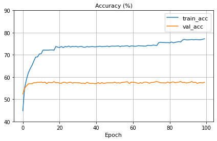
CIFAR10 자체가 그렇게 데이터가 크지 않기 때문에, pretrained model만 활용하기에 적합하지는 않은 것 같다.
conv layer를 변형하거나 Data augmentation 등 여러가지를 시도해 볼 수 있을 것이다. 본 포스팅에서는 pytorch에서 pretrained model을 활용하여 transfer learning에 적용하는 방법에 대한 내용만 다루기로 하자.
Reference
https://tutorials.pytorch.kr/beginner/transfer_learning_tutorial.html
https://ndb796.tistory.com/552
https://yeseullee0311.medium.com/pytorch-transfer-learning-alexnet-how-to-freeze-some-layers-26850fc4ac7e
https://stackoverflow.com/questions/62523912/how-to-freeze-selected-layers-of-a-model-in-pytorch

댓글남기기