
[GIS] 공간정보 데이터를 자유롭게 변형, 가공, 처리하기
업데이트:
개요
![]()
이전 포스팅에서 이어서, 서울특별시 시군구 영역(polyhon)과 소방안전센터(Point)위치 정보를 활영하여 공간 분석에 활용되는 다양한 처리 및 분석기법들을 알아보자.
import pandas as pd
import geopandas as gpd
from shapely.geometry import Point, Polygon, LineString
import matplotlib.pyplot as plt
import matplotlib
import matplotlib.font_manager as fm
font_name = fm.FontProperties(fname = 'C:/Windows/Fonts/malgun.ttf').get_name()
matplotlib.rc('font', family = font_name)

seoul_area = gpd.GeoDataFrame.from_file('data/LARD_ADM_SECT_SGG_11.shp', encoding='cp949')
pt_119 = pd.read_csv('data/서울시 안전센터관할 위치정보 (좌표계_ WGS1984).csv', encoding='cp949', dtype=str)
pt_119['경도'] = pt_119['경도'].astype(float)
pt_119['위도'] = pt_119['위도'].astype(float)
pt_119['geometry'] = pt_119.apply(lambda row : Point([row['경도'], row['위도']]), axis=1)
pt_119 = gpd.GeoDataFrame(pt_119, geometry='geometry')
pt_119.crs = {'init':'epsg:4326'}
pt_119 = pt_119.to_crs({'init':'epsg:5179'})
1. 객체 속성
area: 면적 계산length: 길이 계산boundary: 테두리(LineString객체)exterior: 테두리(LinearRing객체)centroid: 무게중심점xy: 좌표 반환(array, tuple 객체)coords: 좌표 반환(shapely.coords객체)is_valid: 도형 유효성 검사(boolean)geom_type: 공간 객체 타입
area
# area
seoul_area.geometry.area.head()
0    2.453758e+07
1    3.383061e+07
2    3.946631e+07
3    4.685083e+07
4    2.954112e+07
dtype: float64
length
# length
seoul_area.geometry.length.head()
0    24029.227412
1    30532.219899
2    35504.681042
3    43978.564653
4    27448.698426
dtype: float64
polygon의 length는 테두리의 길이(둘레)가 될 것이다.
boundary
# boundary
seoul_area.geometry[0].boundary

boundary는 polygon객체의 테두리로 Linestring객체를 반환한다.
centroid
# centroid
seoul_area.geometry.centroid.head()
0    POINT (968820.2949617257 1950182.073942499)
1     POINT (965998.687667006 1945219.460300438)
2    POINT (961369.9946055702 1944245.952319755)
3    POINT (958548.9290023139 1941666.567629602)
4      POINT (950951.5822470621 1941050.9467013)
dtype: object
centroid는 다각형의 무게중심점으로 중학교 수학시간에 배웠던 것 같다. 자세한 내용은 여기를 참고
xy와 coords
# xy와 coords
print(pt_119['geometry'][0].xy)
print(pt_119['geometry'][0].coords)
print(list(pt_119['geometry'][0].coords))
(array('d', [944285.7077635808]), array('d', [1947726.3905374545]))
<shapely.coords.CoordinateSequence object at 0x000002EDD9292BC8>
[(944285.7077635808, 1947726.3905374545)]
xy와 coords는 사실 shaply의 공간 객체인 Point와 LineString의 속성이기 때문에 GeoDataFrame과 GeoSeries에 바로 적용할 수 없다.
또한 Polygon의 좌표를 뽑기 위해선 boundary로 Line객체를 만들고 속성을 뽑아야 한다.
is_valid
# is_valid
seoul_area.geometry.is_valid.head()
0     True
1    False
2     True
3     True
4     True
dtype: bool
is_valid는 도형이 유효한지를 검사할 때 사용한다. 공간데이터는 좌표나 제작 출처에 따라서 조금씩 모양이 다르기도 하고, 삐져나오거나 마감처리가 잘 안되어 있거나 한 경우가 있는데 처리하지 않으면 에러가 난다.
위를 보니 index1의 객체가 유효하지가 않다고 나와있다. 밑에서 더 알아보자.
2. 공간 관계
within: 포함되는지 여부contain: 포함하고 있는지 여부intersects: 교차하는지 여부(경계에 닿아 있기만 해도됨)crosses: 교차하는지 여부(내부를 지나가야 함)distance: 두 공간 사이의 직선(최단)거리를 계산한다.
within과 contain
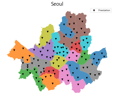
ax = seoul_area.plot(column="SGG_NM", figsize=(8,8), alpha=0.8)
pt_119.plot(ax=ax, marker='v', color='black', label='Firestation')
ax.set_title("Seoul", fontsize=20)
ax.set_axis_off()
plt.legend()
plt.show()
within과 contains는 어법이 반대인 것만 빼면 같은 함수라 할 수 있고 같은 결과를 반환한다.
# 고덕119안전센터는 강동구 안에 있다.
print(pt_119.geometry[17].within(seoul_area.geometry[0]))

# 강동구 안에는 고덕119안전센터가 있다.
print(seoul_area.geometry[0].contains(pt_119.geometry[17]))
True
True
같은 함수인데 왜 저렇게 만들어 뒀냐면, 두 함수 모두 1:1 또는 N:1관계만 입력 가능하고 1:N은 입력이 불가능하다. 따라서 경우에 따라 두 함수 모두 필요할 때가 있다.
- 서울시 119안전센터(N) 중, 강동구(1)에 포함되는 곳은? :
within - 서울시 시군구(N) 중, 고덕안전센터(1)를 포함하는 곳은? :
contains
intersects & crosses
# 강동구와 송파구는 맞닿아 있다.
print(seoul_area.geometry[1].intersects(seoul_area.geometry[1]))

# 하지만 cross 되지는 않는다.
print(seoul_area.geometry[1].crosses(seoul_area.geometry[1]))
True
False
이러한 공간 데이터 간의 관계를 이용해서 다양한 활용이 가능하다.
예를들어 서울시 양천구 내의 소방안전센터 정보를 인덱싱하고 싶다면,
yangcheon_ = seoul_area.loc[seoul_area['SGG_NM']=="양천구",'geometry'].iloc[0]
select_pt = pt_119[pt_119.within(yangcheon_)] #양천구 안에 위치한 소방안전센터 boolean
select_pt
| 고유번호 | 센터ID | 센터명 | 위도 | 경도 | geometry | |
|---|---|---|---|---|---|---|
| 0 | 21 | 1121101 | 양천119안전센터 | 37.527161 | 126.869452 | POINT (944285.7077635808 1947726.390537455) |
| 24 | 31 | 1121105 | 신트리119안전센터 | 37.513474 | 126.851577 | POINT (942695.8419499723 1946218.670628866) |
| 47 | 1 | 1121102 | 신정119안전센터 | 37.520698 | 126.851035 | POINT (942653.4619829537 1947020.444136404) |
| 66 | 65 | 1121104 | 신월119안전센터 | 37.528035 | 126.831056 | POINT (940893.7801357487 1947846.770736765) |
| 74 | 74 | 1121103 | 목동119안전센터 | 37.540990 | 126.876401 | POINT (944909.864544943 1949256.533262795) |
| 101 | 96 | 1117104 | 발산119안전센터 | 37.546084 | 126.829698 | POINT (940788.0721454717 1949850.110233835) |
양천구에는 총 6개의 안전센터가 있네요.
distance
마지막으로 distance는 점과 다각형, 라인 등 두 공간 사이의 직선거리를 계산해준다.
위에서 찾은 안전센터중, 양천안전센터와 발산안전센터 사이의 거리를 구해보자.
# distance
dist = select_pt['geometry'].loc[0].distance(select_pt['geometry'].loc[101])
print("약 %s m" % round(dist))
약 4092 m
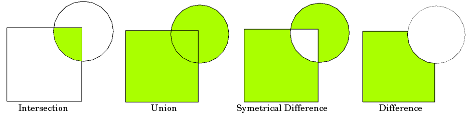
3. 공간 연산 및 변형
buffer: 주어진 거리 내의 모든 점을 이어 Polygon을 만들고(Point,Linestring 적용 시)거나 주어진 거리만큼 확장한다(Polygon 적용 시).envelope: Polygon을 감싸는 가장 작은 사각형 Polygon 객체를 만든다.convexhull: Polygon에 대하여 convex-hull(볼록껍질)을 만든다.unary_union: 여러 공간 데이터의 합집합을 구한다.dissolve: 합집합을 구한다(groupby 기능이 포함).overlay: 합집합,차집합,교집합 등 공간 연산 기능을 제공한다.
buffer는 객체 타입에 상관없이 해당 객체를 감싸는 원형의 반경을 생성해내고, envelope은 Polygon 타입에 대하여 사각형 형태의 반경을 만들어 낸다.
buffer & envelope
# buffer & envelope
yangcheon = pt_119.geometry.iloc[0]
ax = gpd.GeoSeries(yangcheon.buffer(500).envelope).plot(color='skyblue') # envelope
gpd.GeoSeries(yangcheon.buffer(500)).plot(color='pink', ax=ax) # buffer
gpd.GeoSeries(yangcheon).plot(figsize=(5,5), color='black', ax=ax)
plt.title("buffer & envelope")
plt.text(yangcheon.x+100, yangcheon.y, "500m", fontsize=15)
plt.show()
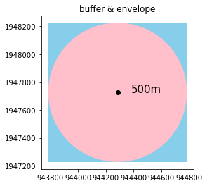
따라서 위와 같은 관계이며, Point에 대하여 500m에 해당하는 사각형 반경을 만들었다고 볼 수도 있다.
초기점에 대하여 grid를 만드는데 유용하게 사용된다.
추가적으로, 위에서 is_valid를 설명할때 송파구가 유효하지 않은 객체임을 확인했었다.
shapefile의 경우 면이나 섬의 경계 등이 깔끔하게 정리되어 있지 않은 경우가 많이 있다. 이런 것을 Topology Error라고 부르며, 다양한 처리방식이 존재한다. 이에 대한 자세한 내용은 추후에 다루기로 하고 여기서는 buffer를 이용하여 보정해보자.
invalid_area = seoul_area.iloc[[1]]
print(invalid_area.is_valid)
print(invalid_area.buffer(0).is_valid) # buffer로 보정
1    False
dtype: bool
1    True
dtype: bool
이렇게 아주 살짝의 buffer만으로도(0도 가능하다) 유효한 객체가 된다(안될경우 조금씩 증가).
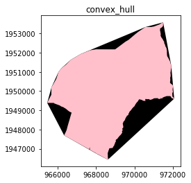
convexhull
convexhull이란 2차원 평면상에 여러개의 점이 있을 때 일부를 이용하여 내부에 모든 점을 포함시키는 다각형을 만드는 것을 의미한다.
(자세한 내용은 여기를 참고하자)
강동구 Polygon으로 확인해보자.
# convex_hull
gangdong = seoul_area.iloc[[0]]
ax = gangdong.convex_hull.plot(color='black')
gangdong.plot(figsize=(5,5), ax=ax, color='pink')
plt.title("convex_hull")
plt.show()
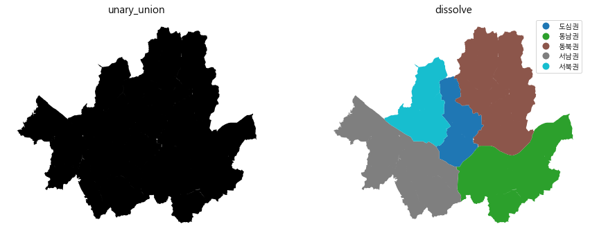
unary_union와 dissolve
이제 unary_union와 dissolve를 알아보기 위해 서울시 생활권 계획에 따른 5개 생활권을 그룹핑해보자.
dict_ = {}
dict_['서남권'] = ["강서구","양천구","구로구","영등포구","금천구","동작구","관악구"]
dict_['동남권'] = ["서초구","강남구","송파구","강동구"]
dict_['서북권'] = ["은평구","마포구","서대문구"]
dict_['도심권'] = ["종로구","중구","용산구"]
dict_['동북권'] = ["서울시도봉구","강북구","서울시노원구","서울시성북구","동대문구","성동구","중랑구","광진구"]
for k,v in dict_.items():
    seoul_area.loc[seoul_area['SGG_NM'].isin(v), 'group'] = k
plt.figure(figsize=(15,15))
ax = plt.subplot(1, 2, 1)
gpd.GeoSeries(seoul_area.unary_union).plot(color='black', ax=ax)
ax.set_title("unary_union", fontsize=15)
ax.set_axis_off()

ax = plt.subplot(1, 2, 2)
seoul_area.dissolve(by='group').reset_index().plot(column = 'group', ax=ax, legend=True)
ax.set_title("dissolve", fontsize=15)
ax.set_axis_off()
overlay
다음은 overlay이다.
공간 연산 규칙의 기본 4가지는 아래와 같다. 이는 개별 객체(Polygon, LineString)에 대한 연산이 아니라 데이터 프레임 전체를 다룰 수 있는 Geopandas 기능이다. 개별 객체에 대한 기능은 shapely의 함수이며 이를 연계하여 Geopandas에서 활용하게 되는 것이다.
Geopandas 공식 org의 예제로 알아보자.
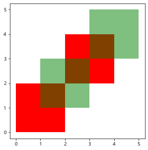
from shapely.geometry import Polygon

polys1 = gpd.GeoSeries([Polygon([(0,0), (2,0), (2,2), (0,2)]),
                               Polygon([(2,2), (4,2), (4,4), (2,4)])])
polys2 = gpd.GeoSeries([Polygon([(1,1), (3,1), (3,3), (1,3)]),
                               Polygon([(3,3), (5,3), (5,5), (3,5)])])
df1 = gpd.GeoDataFrame({'geometry': polys1, 'df1':[1,2]})
df2 = gpd.GeoDataFrame({'geometry': polys2, 'df2':[1,2]})

ax = df1.plot(color='red', figsize=(5,5))
df2.plot(ax=ax, color='green', alpha=0.5)
plt.show()
res_union = gpd.overlay(df1, df2, how='union')
print(res_union)
res_union = res_union.reset_index()
res_union['index'] = res_union['index'].astype(str)

ax = res_union.plot(column='index', legend=True, figsize=(5,5))
df1.plot(ax=ax, facecolor='none', edgecolor='k')
df2.plot(ax=ax, facecolor='none', edgecolor='k')
plt.title("union", fontsize=15)
plt.show()
   df1  df2                                           geometry
0  1.0  1.0                POLYGON ((1 2, 2 2, 2 1, 1 1, 1 2))
1  2.0  1.0                POLYGON ((2 2, 2 3, 3 3, 3 2, 2 2))
2  2.0  2.0                POLYGON ((3 4, 4 4, 4 3, 3 3, 3 4))
3  1.0  NaN      POLYGON ((0 0, 0 2, 1 2, 1 1, 2 1, 2 0, 0 0))
4  2.0  NaN  (POLYGON ((2 3, 2 4, 3 4, 3 3, 2 3)), POLYGON ...
5  NaN  1.0  (POLYGON ((1 2, 1 3, 2 3, 2 2, 1 2)), POLYGON ...
6  NaN  2.0      POLYGON ((3 4, 3 5, 5 5, 5 3, 4 3, 4 4, 3 4))
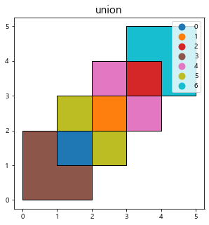
보다시피 df1과 df2는 각각 2개의 Polygon을 가지고 있었고(총 4개), Union 결과 경계를 따라 7개의 Polygon데이터로 분할된 것을 알 수 있다. 주의할 점은 4번과 5번 Polygon은 개별 사각형으로 분리되지 않고 2개의 작은 사각형(MultiPolygon)이 되었다.
모두 분리된 객체가 필요하다면 MultiPolygon도 분리해주는 과정까지 거쳐야 한다.
res_intersection = gpd.overlay(df1, df2, how='intersection')
print(res_intersection)

ax = res_intersection.plot(figsize=(5,5),cmap='tab10')
df1.plot(ax=ax, facecolor='none', edgecolor='k')
df2.plot(ax=ax, facecolor='none', edgecolor='k')
plt.title("Intersection", fontsize=15)
plt.show()
   df1  df2                             geometry
0    1    1  POLYGON ((1 2, 2 2, 2 1, 1 1, 1 2))
1    2    1  POLYGON ((2 2, 2 3, 3 3, 3 2, 2 2))
2    2    2  POLYGON ((3 4, 4 4, 4 3, 3 3, 3 4))
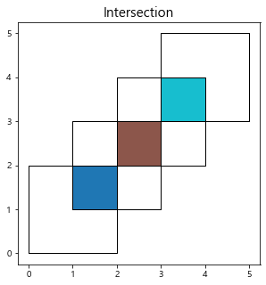
Intersection은 공집합에 해당하는 Polygon데이터를 추출한다.
printres_symdiff = gpd.overlay(df1, df2, how='symmetric_difference')
print(printres_symdiff)

ax = printres_symdiff.plot(figsize=(5,5),cmap='tab10')
df1.plot(ax=ax, facecolor='none', edgecolor='k')
df2.plot(ax=ax, facecolor='none', edgecolor='k')
plt.title("symmetric_difference", fontsize=15)
plt.show()
   df1  df2                                           geometry
0  1.0  NaN      POLYGON ((0 0, 0 2, 1 2, 1 1, 2 1, 2 0, 0 0))
1  2.0  NaN  (POLYGON ((2 3, 2 4, 3 4, 3 3, 2 3)), POLYGON ...
2  NaN  1.0  (POLYGON ((1 2, 1 3, 2 3, 2 2, 1 2)), POLYGON ...
3  NaN  2.0      POLYGON ((3 4, 3 5, 5 5, 5 3, 4 3, 4 4, 3 4))
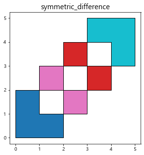
symmetric_difference는 여집합(합집합-교집합)에 해당하는 Polygon 데이터를 추출한다.
res_difference = gpd.overlay(df1, df2, how='difference')
print(res_difference)

ax = res_difference.plot(figsize=(5,5),cmap='tab10')
df1.plot(ax=ax, facecolor='none', edgecolor='k')
df2.plot(ax=ax, facecolor='none', edgecolor='k')
plt.title("difference", fontsize=15)
plt.show()
                                            geometry  df1
0      POLYGON ((0 0, 0 2, 1 2, 1 1, 2 1, 2 0, 0 0))    1
1  (POLYGON ((2 3, 2 4, 3 4, 3 3, 2 3)), POLYGON ...    2
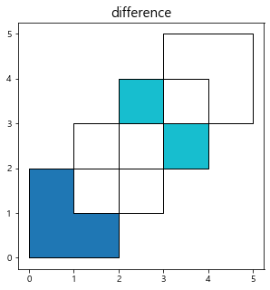
difference는 전자(df1)에서 후자(df2)의 차집합에 해당하는 Polygon 데이터를 추출한다.
3. 정리
이제 다시 서울시 시군구별 shp와, 119소방안전센터 데이터로 배운것을 활용해보며 마무리해보자.
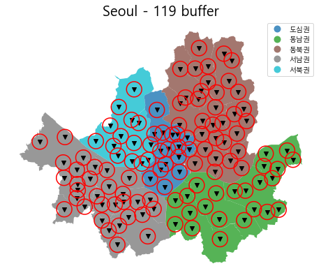
- 119소방안전센터의 반경 1km를 그린다.
- 서울시에서 해당 반경으로 커버되지 않는 부분을 구한다.
- 생활권별 미커버 면적을 계산한다.
buf_poly = gpd.GeoDataFrame({'geometry': pt_119.buffer(1000)})
origin_ = seoul_area.groupby(['group']).apply(lambda gr : gr.area.sum())

ax = seoul_area.plot(column="group", figsize=(8,8), alpha=0.8, legend=True)
pt_119.plot(ax=ax, marker='v', color='black', label='Firestation')
buf_poly.boundary.plot(ax=ax, color='red')
ax.set_title("Seoul - 119 buffer", fontsize=20)
ax.set_axis_off()
plt.show()

print(origin_)
group
도심권    5.582471e+07
동남권    1.446853e+08
동북권    1.710378e+08
서남권    1.623935e+08
서북권    7.129826e+07
dtype: float64
dif_area = gpd.overlay(seoul_area, buf_poly, how='difference')
dif_area = dif_area.dissolve(by='group')
ax = dif_area.plot(column="SGG_NM", figsize=(8,8), alpha=0.8)
ax.set_title("Seoul - 119 buffer", fontsize=20)
ax.set_axis_off()
plt.show()

print("전체 대비 미커버지역 비율")
print(round(dif_area.area / origin_ * 100))
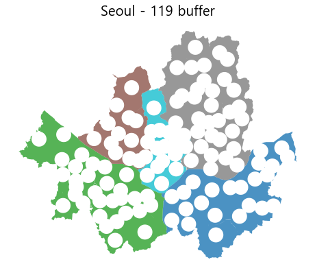
전체 대비 미커버지역 비율
group
도심권    29.0
동남권    53.0
동북권    45.0
서남권    47.0
서북권    48.0
dtype: float64

댓글남기기