
[pytorch] Tensor와 Autograd, 그리고 간단한 Neural Network
업데이트:
개요

이번 포스팅은 pytorch kr의 tutorial 중 하나인 “Pytorch로 딥러닝하기: 60분만에 끝장내기“를 따라해보며 공부한 내용입니다.
1. 텐서(Tensor)
import torch
import numpy as np
1.1 Tensor 생성
data = [[1,2],[3,4]]
x_data = torch.tensor(data)
print(x_data)
tensor([[1, 2],
        [3, 4]])
np_array = np.array(data)
#x_np = torch.tensor(np_array)
x_np = torch.from_numpy(np_array)
print(x_np)
tensor([[1, 2],
        [3, 4]], dtype=torch.int32)
# 다른 tensor의 shape과 dtype을 유지하면서, 1이나 0으로 채워진 텐서배열 생성
x_ones = torch.ones_like(x_data)
x_zeros = torch.zeros_like(x_data)
print(x_ones)
print(x_zeros)
print()

# shape는 유지, dtype은 float으로 수정, random 배열로 변경
x_rand = torch.rand_like(x_data, dtype=torch.float)
print(x_rand)
tensor([[1, 1],
        [1, 1]])
tensor([[0, 0],
        [0, 0]])

tensor([[0.9445, 0.3262],
        [0.1734, 0.3048]])
# 차원(shape)에 따른 random이나 0 or 1값으로 채워진 텐서배열
shape = (2, 3,)
rand_tensor = torch.rand(shape)
ones_tensor = torch.ones(shape)
zeros_tensor = torch.zeros(shape)

print(f"Random Tensor: \n {rand_tensor} \n")
print(f"Ones Tensor: \n {ones_tensor} \n")
print(f"Zeros Tensor: \n {zeros_tensor}")
Random Tensor:
 tensor([[0.3344, 0.0342, 0.6235],
        [0.8186, 0.2232, 0.8440]])

Ones Tensor:
 tensor([[1., 1., 1.],
        [1., 1., 1.]])

Zeros Tensor:
 tensor([[0., 0., 0.],
        [0., 0., 0.]])
1.2 텐서의 속성(Attribute)
tensor = torch.rand(3,4)
print("shape:",tensor.shape)
print("data type:",tensor.dtype)
print("device:",tensor.device)
shape: torch.Size([3, 4])
data type: torch.float32
device: cpu
1.3 텐서 연산(Operation)
- GPU할당 여부를 확인
if torch.cuda.is_available():
  tensor = tensor.to('cuda')
  print(f"Device tensor is stored on: {tensor.device}")
Device tensor is stored on: cuda:0
- Tensor 인덱싱하기
tensor = torch.ones(4,4)
print(tensor)
tensor[:,1]=0
print(tensor)
tensor([[1., 1., 1., 1.],
        [1., 1., 1., 1.],
        [1., 1., 1., 1.],
        [1., 1., 1., 1.]])
tensor([[1., 0., 1., 1.],
        [1., 0., 1., 1.],
        [1., 0., 1., 1.],
        [1., 0., 1., 1.]])
- Tensor 합치기
# 가로로 합치기
t1 = torch.cat([tensor, tensor, tensor], dim=1)
print(t1)

# 세로로 합치기
t2 = torch.cat([tensor, tensor, tensor], dim=0)
print(t2)
tensor([[1., 0., 1., 1., 1., 0., 1., 1., 1., 0., 1., 1.],
        [1., 0., 1., 1., 1., 0., 1., 1., 1., 0., 1., 1.],
        [1., 0., 1., 1., 1., 0., 1., 1., 1., 0., 1., 1.],
        [1., 0., 1., 1., 1., 0., 1., 1., 1., 0., 1., 1.]])
tensor([[1., 0., 1., 1.],
        [1., 0., 1., 1.],
        [1., 0., 1., 1.],
        [1., 0., 1., 1.],
        [1., 0., 1., 1.],
        [1., 0., 1., 1.],
        [1., 0., 1., 1.],
        [1., 0., 1., 1.],
        [1., 0., 1., 1.],
        [1., 0., 1., 1.],
        [1., 0., 1., 1.],
        [1., 0., 1., 1.]])
- 텐서 곱하기: 원소 간 곱(element-wise product)
print(tensor.mul(tensor))
print(tensor * tensor)
tensor([[1., 0., 1., 1.],
        [1., 0., 1., 1.],
        [1., 0., 1., 1.],
        [1., 0., 1., 1.]])
tensor([[1., 0., 1., 1.],
        [1., 0., 1., 1.],
        [1., 0., 1., 1.],
        [1., 0., 1., 1.]])
- 텐서 곱하기: 행렬곱(matrix multiplication)
print(tensor.matmul(tensor))
print(tensor @ tensor)
tensor([[3., 0., 3., 3.],
        [3., 0., 3., 3.],
        [3., 0., 3., 3.],
        [3., 0., 3., 3.]])
tensor([[3., 0., 3., 3.],
        [3., 0., 3., 3.],
        [3., 0., 3., 3.],
        [3., 0., 3., 3.]])
- 텐서 더하기
t_add = tensor+5
print(t_add)
print(tensor.add(5))

# in_place 연산 (바로 바꿔치기)
print(t_add.add_(5))
print(t_add)
tensor([[6., 5., 6., 6.],
        [6., 5., 6., 6.],
        [6., 5., 6., 6.],
        [6., 5., 6., 6.]])
tensor([[6., 5., 6., 6.],
        [6., 5., 6., 6.],
        [6., 5., 6., 6.],
        [6., 5., 6., 6.]])
tensor([[11., 10., 11., 11.],
        [11., 10., 11., 11.],
        [11., 10., 11., 11.],
        [11., 10., 11., 11.]])
tensor([[11., 10., 11., 11.],
        [11., 10., 11., 11.],
        [11., 10., 11., 11.],
        [11., 10., 11., 11.]])
1.4 Numpy 변환
t = torch.ones(5)
print(t)
t_np = t.numpy()
print(t_np)
tensor([1., 1., 1., 1., 1.])
[1. 1. 1. 1. 1.]
# tensor에 in-place를 해주면 numpy에 바로 반영됨
t.add_(5)
print(t_np)
[6. 6. 6. 6. 6.]
# 반대도 마찬가지임
np.add(t_np, 1, out=t_np)
print(t)
tensor([7., 7., 7., 7., 7.])
2. 미분 연산을 지원하는 torch.autograd
2.1 pytorch에서 사용법
torchvision에서는 다양한 pretrained model을 기본적으로 제공한다.
- resnet18 로딩
import torch, torchvision
model = torchvision.models.resnet18(pretrained=True)
data = torch.rand(1, 3, 64, 64)
labels = torch.rand(1, 1000)
- prediction 생성 (forward pass)
prediction = model(data)
print(prediction.shape)
print(prediction[0][0])
torch.Size([1, 1000])
tensor(-0.5587, grad_fn=<SelectBackward0>)
- loss 계산 (sum)
# sum으로 계산하면 자동으로 grad_fn이 SumBackward0로 들어감
loss = (prediction - labels).sum()
loss
tensor(-493.2259, grad_fn=<SumBackward0>)
backward()를 통해 backpropagation 하면.grad속성에 gradient를 저장해준다.
loss.backward()
- 다음은 Optimizer를 불러오고 모델의 parameter를 등록해주는 과정이다.
optim = torch.optim.SGD(model.parameters(), lr=1e-2, momentum=0.9)
- 마지막으로
.step을 통해 경사하강법을 수행한다.
앞서 backward()로 저장했던, gradient와 위의 learning rate, momentum 등에 따라 실질적으로 파라미터를 갱신시켜주는 것으로 이해하면 된다.
optim.step()
아래와 같이 동일한 데이터로 inference하면 prediction 값이 바뀌어 있음을 확인할 수 있다.
prediction = model(data)
print(prediction[0][0])
tensor(-5.0230, grad_fn=<SelectBackward0>)
2.2 Autograd에서 미분(differentiation)
위에서 구현한 바를 autograd가 어떻게 미분을 하는지 좀더 직관적으로 알아보자.
- 먼저 2개의 tensor를 생성한다.
*requires_grad=True는 autograd가 연산들을 기록하도록 명시하는 설정(미분을 위해)이다.
import torch

a = torch.tensor([2., 3.], requires_grad=True)
b = torch.tensor([6., 4.], requires_grad=True)
간단한 Loss function이 아래와 같다고 가정해보자.
(즉, a와 b는 파라미터이고 Q는 loss function임)
Q=3*a**3-b**2
이제 각 파라미터에 대한 gradient를 계산하려면 아래와 같이 미분해야한다.
따라서 backward()함수가 이 값을 실제로 저장하는지 확인할 것이다.
\(\frac {dQ}{da}=9a^2\) \(\frac {dQ}{db}=-2b\)
Q.sum().backward()
print(a.grad)
print(b.grad)
tensor([36., 81.])
tensor([-12.,  -8.])
일반적으로는 위와 같이 집계된 스칼라(scalar)값에 대해 backward()를 하는데,
출력 y값이 단일값이 아니라 벡터(Vector)인 경우는 차원을 유지해주어야한다.
이를 위해 pytorch에서는 JVP (Jacobian Vector Product)를 이용한다.
자세한 내용은 여기를 참고
external_grad = torch.tensor([1., 1.])
Q.backward(gradient=external_grad)
print(a.grad)
print(b.grad)
tensor([36., 81.])
tensor([-12.,  -8.])
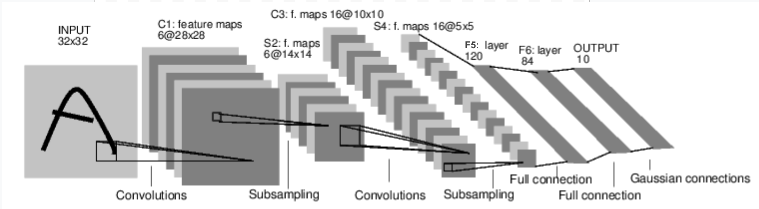
3. 신경망 (Neural Networks)
아래와 같이 이미지(mnist 데이터)를 학습하고 숫자를 분류하는 신경망을 만들어보자.
신경망의 일반적인 학습과정은 아래와 같다.
- 학습 가능한 매개변수(또는 가중치(weight))를 갖는 신경망 정의
- 데이터셋(dataset) 입력을 반복
- 입력을 신경망에서 전파(process)
- 손실(loss; 출력이 정답으로부터 얼마나 떨어져있는지) 계산
- 변화도(gradient)를 신경망의 매개변수들에 역전파
- 가중치 업데이트
(가중치 업데이트의 일반적인 방법: 새로운 가중치(weight) = 가중치(weight) - 학습률(learning rate) * 변화도(gradient))
3.1 신경망 정의
pytorch의 신경망 layer들이 갖고 있는 인자들은 기본적으로, 입력 차원 수(in_features)와 출력 차원 수(out_features)를 입력하도록 구성되어 있다.
따라서 이전 layer의 출력과 다음 layer의 입력이 같도록 차원을 맞춰주어야한다.
그리고 CNN 구현 시에는 channel, kernel(filter) 개념이 추가되어 아래와 같이 정의해주어야 한다.
nn.conv2d(in_channels, out_channels, kernel_size)
따라서 다음 출력 차원에 맞도록 계산해서 넣어주자.
import torch
import torch.nn as nn
import torch.nn.functional as F

class Net(nn.Module):

    def __init__(self):
        super(Net, self).__init__()
        # [배치크기 x 채널 x 높이(height) x 너비(width)]
        # [1,1,32,32] -> [1,6,28,28]
        # [1,6,28,28] -> [1,6,14,14] max pool2d(2) 하면 가로세로가 각각 반으로 줄어듦
        self.conv1 = nn.Conv2d(1, 6, 5)
        # [1,6,14,14] -> [1,16,10,10]
        # [1,16,10,10] -> [1,16,5,5] max pool2d(2)
        self.conv2 = nn.Conv2d(6, 16, 5)
        # 아핀(affine) 연산: y = Wx + b
        # [1,16*5*5] -> [1,120]
        self.fc1 = nn.Linear(16 * 5 * 5, 120)  # 5*5은 이미지 차원에 해당
        # [1,120] -> [1,84]
        self.fc2 = nn.Linear(120, 84)
        # [1,84] -> [1,10]
        self.fc3 = nn.Linear(84, 10)

    def forward(self, x):
        # (2, 2) 크기 윈도우에 대해 맥스 풀링(max pooling)
        x = F.max_pool2d(F.relu(self.conv1(x)), (2, 2))
        # 크기가 제곱수라면, 하나의 숫자만을 특정(specify)
        x = F.max_pool2d(F.relu(self.conv2(x)), 2)
        x = torch.flatten(x, 1) # 배치 차원을 제외한 모든 차원을 하나로 평탄화(flatten)
        x = F.relu(self.fc1(x))
        x = F.relu(self.fc2(x))
        x = self.fc3(x)
        return x

net = Net()
print(net)
Net(
  (conv1): Conv2d(1, 6, kernel_size=(5, 5), stride=(1, 1))
  (conv2): Conv2d(6, 16, kernel_size=(5, 5), stride=(1, 1))
  (fc1): Linear(in_features=400, out_features=120, bias=True)
  (fc2): Linear(in_features=120, out_features=84, bias=True)
  (fc3): Linear(in_features=84, out_features=10, bias=True)
)
- 학습 가능한 신경망의 파라미터 출력(현재는 초기 weight)
params = list(net.parameters())
print(len(params))
print(params[0].size())  # conv1의 .weight
10
torch.Size([6, 1, 5, 5])
input = torch.randn(1, 1, 32, 32) # [배치크기 x 채널 x 높이(height) x 너비(width)]
out = net(input)
print(out)
tensor([[ 0.0019, -0.1036, -0.0823,  0.1105,  0.0220,  0.0391,  0.0724,  0.0751,
         -0.0191, -0.1104]], grad_fn=<AddmmBackward0>)
net.zero_grad()
out.backward(torch.randn(1, 10))
3.2 손실 함수(Loss function)
nn에 여러가지 손실 함수를 제공해주고 있다.
여기서는 평균제곱오차를 계산해주는 nn.MSELoss()를 사용한다.
output = net(input)
target = torch.randn(10)  # 예시를 위한 임의의 정답
target = target.view(1, -1)  # 출력과 같은 shape로 만듦
criterion = nn.MSELoss()

loss = criterion(output, target)
print(loss)
tensor(0.5878, grad_fn=<MseLossBackward0>)
grad_fn인자를 활용하여 backpropagation되는 단계들을 추적해볼 수도 있다.
위에서 디자인 했던 신경망 구조의 반대방향으로 역전파가 발생하는 것을 확인할 수 있다.
print(loss.grad_fn)
print(loss.grad_fn.next_functions[0][0])
print(loss.grad_fn.next_functions[0][0].next_functions[1][0])
print(loss.grad_fn.next_functions[0][0].next_functions[1][0].next_functions[0][0])
print(loss.grad_fn.next_functions[0][0].next_functions[1][0].next_functions[0][0].next_functions[1][0])
print(loss.grad_fn.next_functions[0][0].next_functions[1][0].next_functions[0][0].next_functions[1][0].next_functions[0][0])
print(loss.grad_fn.next_functions[0][0].next_functions[1][0].next_functions[0][0].next_functions[1][0].next_functions[0][0].next_functions[1][0])
print(loss.grad_fn.next_functions[0][0].next_functions[1][0].next_functions[0][0].next_functions[1][0].next_functions[0][0].next_functions[1][0].next_functions[0][0])
<MseLossBackward0 object at 0x000001A837ABEF88>
<AddmmBackward0 object at 0x000001A837ABE4C8>
<ReluBackward0 object at 0x000001A837ABE4C8>
<AddmmBackward0 object at 0x000001A8379EF648>
<ReluBackward0 object at 0x000001A837ABE4C8>
<AddmmBackward0 object at 0x000001A8379CEB48>
<ReshapeAliasBackward0 object at 0x000001A837ABEF88>
<MaxPool2DWithIndicesBackward0 object at 0x000001A8379CEB48>
3.3 역전파(Backpropagation)
zero_grad()를 명시해주어야하는 이유는 다음과 같다.
기본적으로 미니배치와 루프(epoch)를 이용해서 학습이 반복되는데, 한 epoch이 끝나면 gradient를 0으로 초기화(zero_grad) 시켜주어야한다.
그런데, 새로운 epoch에서의 gradient가 이전 epoch에 누적되면 현재 gradient 값에 영향을 주어 제대로 학습이 되지 않기 때문이다.
net.zero_grad()     # 모든 매개변수의 변화도 버퍼를 0으로 만듦

print('conv1.bias.grad before backward')
print(net.conv1.bias.grad)

loss.backward()

print('conv1.bias.grad after backward')
print(net.conv1.bias.grad)
conv1.bias.grad before backward
tensor([0., 0., 0., 0., 0., 0.])
conv1.bias.grad after backward
tensor([ 0.0072, -0.0048, -0.0158,  0.0011,  0.0010, -0.0047])
3.4 가중치 갱신
앞서 언급한 것처럼 실제로 가장 많이 사용하는 방법(가중치 업데이트)은 확률적 경사하강법(SGD: Stochastic Gradient Descent)이다.
아래와 같이 weight을 업데이트한다.
새로운 가중치(weight) = 가중치(weight) - 학습률(learning rate) * 변화도(gradient)
단순하게 python으로 구현하면 아래와 같이 직접 갱신해줄 수도 있다.
learning_rate = 0.01
for f in net.parameters():
    f.data.sub_(f.grad.data * learning_rate)
pytorch에서는 torch.optim을 제공해서, SGD 외에도 Nesterov-SGD, Adam, RMSProp 등을 간편하게 이용할 수 있다.
import torch.optim as optim

# Optimizer를 생성합니다.
optimizer = optim.SGD(net.parameters(), lr=0.01)

# 학습 과정(training loop)은 다음과 같습니다:
optimizer.zero_grad()   # gradient 를 0으로 초기화
output = net(input)
loss = criterion(output, target)
loss.backward()
optimizer.step()    # 업데이트 진행
Reference
https://tutorials.pytorch.kr/beginner/deep_learning_60min_blitz.html
https://hongl.tistory.com/273
https://velog.io/@kjb0531/zerograd%EC%9D%98-%EC%9D%B4%ED%95%B4

댓글남기기