
[Handson ML] 분류(Classification)
업데이트:
개요

이번 포스팅에서는 MNIST 데이터셋을 활용하여 분류(classification) 문제를 다뤄보자.
1. MNIST
- MNIST란, 손으로 쓴 숫자들의 이미지를 모아놓은 데이터를 의미한다.
- 70,000개의 작은 숫자 이미지와 각 이미지가 어떤 숫자를 나타내는지 레이블 되어 있는 데이터로 머신러닝 딥러닝 알고리즘의 학습데이터로 많이 사용되는 유명한 데이터 셋이다.
- 변수 : 784(28x28픽셀)개
- 변수 값 : 0(흰색) ~ 255(검은색)까지의 픽셀 강도
import pandas as pd
import numpy as np
import matplotlib
import matplotlib.pyplot as plt
def sort_by_target(mnist):
    reorder_train = np.array(sorted([(target, i) for i, target in enumerate(mnist.target[:60000])]))[:, 1]
    reorder_test = np.array(sorted([(target, i) for i, target in enumerate(mnist.target[60000:])]))[:, 1]
    mnist.data[:60000] = mnist.data[reorder_train]
    mnist.target[:60000] = mnist.target[reorder_train]
    mnist.data[60000:] = mnist.data[reorder_test + 60000]
    mnist.target[60000:] = mnist.target[reorder_test + 60000]
from sklearn.datasets import fetch_openml
mnist = fetch_openml('mnist_784', version=1, cache=True)
mnist.target = mnist.target.astype(np.int8) # fetch_openml() returns targets as strings
sort_by_target(mnist) # fetch_openml() returns an unsorted dataset
dir(mnist)
['DESCR', 'categories', 'data', 'details', 'feature_names', 'target', 'url']
이 mnist 데이터는 딕셔너리와 비슷한 구조를 가지고 있다.
- 데이터셋을 설명하는 DESCR 키
- 샘플이 하나의 행, 특성이 하나의 열로 구성된 배열을 가진 data키
- 레이블의 배열을 담고 있는 targe키
X, y = mnist["data"], mnist["target"]
이 데이터를 살펴보면 이미지가 70,000개가 있고, 각 이미지에는 784개의 특성이 있다.
이는 특성이 784(28x28)개인 이유는 이미지가 28x28 픽셀이기 때문이다.
print(X.shape)
print(y.shape)
(70000, 784)
(70000,)
데이터 셋에서 이미지 하나(row한개)를 확인해 보자.
784개의 원소를 가진 1차원 배열을 reshape를 이용해 28x28의 2차원 배열로 만들어 imshow()함수를 활용해 그릴 수 있다.
some_digit = X[36000]
some_digit_image = some_digit.reshape(28,28)


plt.imshow(some_digit_image, cmap = matplotlib.cm.binary,
          interpolation="nearest")
plt.axis("off")
plt.show()

이미지가 숫자 5처럼 보이는데 target값을 확인해보면 실제로 5인 것을 알 수 있다.
y[36000]
5
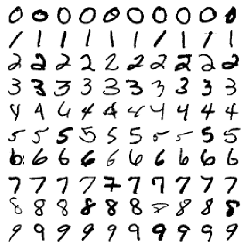
더 많은 이미지를 한번 그려보자(100개).
def plot_digits(instances, images_per_row=10, **options):
    size = 28
    images_per_row = min(len(instances), images_per_row)                      # 행 1개당 이미지 수 지정
    images = [instance.reshape(size,size) for instance in instances]         # 행 하나하나 for문으로 2차원 배열 만들기
    n_rows = (len(instances) - 1) // images_per_row + 1                      # 행의 수 지정
    row_images = []
    n_empty = n_rows * images_per_row - len(instances)
    images.append(np.zeros((size, size * n_empty)))
    for row in range(n_rows):
        rimages = images[row * images_per_row : (row + 1) * images_per_row]
        row_images.append(np.concatenate(rimages, axis=1))
    image = np.concatenate(row_images, axis=0)
    plt.imshow(image, cmap = matplotlib.cm.binary, **options)
    plt.axis("off")
plt.figure(figsize=(9,9))
example_images = np.r_[X[:12000:600], X[13000:30600:600], X[30600:60000:590]]
plot_digits(example_images, images_per_row=10)
plt.show()
이제 train, test셋을 만들고 작업을 시작해보자!
X_train, X_test, y_train, y_test = X[:60000], X[60000:], y[:60000], y[60000:]
train데이터는 섞어서 훈련 샘플의 순서에 영향이 없더록 해주자.
np.random.seed(7)
shuffle_index = np.random.permutation(60000)
X_train, y_train = X_train[shuffle_index], y_train[shuffle_index]
2. 이진분류기(Binary classifier) 훈련
문제를 단순화 해서 5를 식별하는 분류기(5면 O, 아니면 X)를 만들어 보자.
# boolean으로, 5면 True 아니면 False
y_train_5 = (y_train == 5)
y_test_5 = (y_test == 5)
사이킷런의 SGDClassifier클래스를 사용한 확률적 경사 하강법(SGD, Stochastic Gradient Descent) 분류기를 만들어보자.
전체 훈련데이터를 이용해 종속변수(True or False)를 예측하도록 훈련시켜보자.
from sklearn.linear_model import SGDClassifier

sgd_clf = SGDClassifier(max_iter = 5, random_state=42)
sgd_clf.fit(X_train, y_train_5)
SGDClassifier(alpha=0.0001, average=False, class_weight=None,
              early_stopping=False, epsilon=0.1, eta0=0.0, fit_intercept=True,
              l1_ratio=0.15, learning_rate='optimal', loss='hinge', max_iter=5,
              n_iter_no_change=5, n_jobs=None, penalty='l2', power_t=0.5,
              random_state=42, shuffle=True, tol=0.001, validation_fraction=0.1,
              verbose=0, warm_start=False)
분류기가 제대로 5를 분류하는데 실패했다.
sgd_clf.predict([some_digit]) # 아까 샘플로 확인했던 숫자 5
array([False])
3. 성능측정
3-1. 교차 검증을 사용한 정확도 측정
사이킷런에서 제공하는 cross_val_score()함수와 같은 기능을 하는 교차 검증 코드를 먼저 구현해보자.
from sklearn.model_selection import StratifiedKFold
from sklearn.base import clone

skfolds = StratifiedKFold(n_splits=3, random_state=42)     # 계층적 샘플링을 해주는 변환기 생성

for train_index, test_index in skfolds.split(X_train, y_train_5):   # 3겹이므로, 3쌍(train, test)의 인덱스를 반환
    clone_clf = clone(sgd_clf)          # 앞서 만든 모델 clone
    X_train_folds = X_train[train_index]      # x_train데이터 인덱싱
    y_train_folds = (y_train_5[train_index])  # y_train데이터 인덱싱
    X_test_fold = X_train[test_index]         # x_test데이터 인덱싱
    y_test_fold = (y_train_5[test_index])     # y_test데이터 인덱싱

    clone_clf.fit(X_train_folds, y_train_folds)  # 모델 학습
    y_pred = clone_clf.predict(X_test_fold)      # 모델 적합값(True or False)
    n_correct = sum(y_pred == y_test_fold)       # 실제값과 비교
    print(n_correct / len(y_pred))               # 전체 값 대비 분류된 값
0.949
0.96785
0.9649
여기서 헷갈리지 말아야 할 점은(난 헷갈린다..), k-fold교차 검증을 시행할때의 test 데이터는 처음에 분할했던 테스트 데이터가 아니다.
그러니까 총 70000개의 데이터를 훈련데이터 60000개, 테스트데이터 10000개로 나누었고.
이 훈련데이터(60000개)를 다시 3등분(20000개 씩)해서 훈련데이터40000개, 테스트데이터 20000개로 교차검증을 실시하는 것이다.
이번에는 사이킷런에서 제공하는 cross_val_score()함수를 이용해보자.
from sklearn.model_selection import cross_val_score
cross_val_score(sgd_clf, X_train, y_train_5, cv=3, scoring="accuracy")
array([0.949 , 0.96785, 0.9649 ])
정확도가 굉장히 높게 나왔다.
그럼 이번에는 모든 이미지를 5가 아니라고 해버리는 더미 분류기를 만들어 비교해보자.
from sklearn.base import BaseEstimator

class Never5Classifier(BaseEstimator):
    def fit(self, X, y=None):
        pass
    def predict(self,X):
        return np.zeros((len(X),1), dtype=bool)
여기서 dtype=bool옵션은 0이면 False, 1이면 True를 반환해주는데, np.zeros()함수는 모든 숫자를 0으로 채워주므로 모두 False가 삽입된다.
즉, 모두 5가 아님(False)을 나타내는 분류기인 것이다.
never_5_clf = Never5Classifier()
cross_val_score(never_5_clf, X_train, y_train_5, cv =3, scoring = "accuracy")
array([0.91075, 0.90555, 0.91265])
실제로 5가 모두 아니라고만 예측해도, 정확도가 90%이상이 나온다.
이는 불균형 데이터 셋(비율이 적절하게 분포하지 않음)의 경우 왜곡된 결과를 초래할 수 있다.
never_5_clf = Never5Classifier()
never_5_clf.fit(X_train, y_train_5)
n_correct = sum(never_5_clf.predict(X_train) == y_train_5.reshape(-1,1))
print(n_correct / len(y_train_5))
[0.90965]
(y_train_5==False).sum() / len(y_train_5)
0.90965
이건 그냥 해본 것..
5가 아닌것 자체가 90.965%이다.
3-2. 오차 행렬(Confusion Matrix)
from sklearn.model_selection import cross_val_predict

y_train_pred = cross_val_predict(sgd_clf, X_train, y_train_5, cv=3)
from sklearn.metrics import confusion_matrix
confusion_matrix(y_train_5, y_train_pred)
array([[53148,  1431],
       [  934,  4487]], dtype=int64)
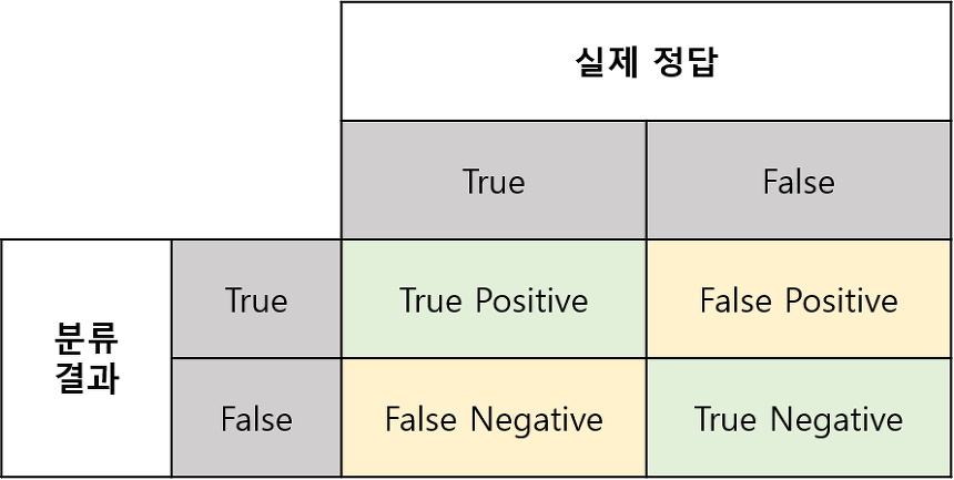
출처 : https://sumniya.tistory.com/26
행은 실제값, 열은 예측값을 나타낸다.
- 1행1열(53148) : ‘5아님’을 ‘5아님’으로 맞게 분류
- 1행2열(1431) : ‘5아님’을 ‘5맞음’으로 잘못 분류
- 2행1열(934) : ‘5맞음’을 ‘5아님’으로 잘못 분류
- 2행2열(4487) : ‘5맞음’을 ‘5맞음’으로 맞게 분류
즉, 100%완벽한 분류기는 행렬의 대각원소 값들 외에는 0이 된다.
3-3. 정밀도(precision)와 재현율(recall)
정밀도(precision) : TP / (TP + FP)
분류기가 양성으로 분류한 값들 중 진짜 양성의 비율을 의미
재현율(recall) 또는 민감도(sensitivity) : TP / (TP + FN)
양성인 실제 값들 중 분류기가 양성으로 분류한 비율을 의미
from sklearn.metrics import precision_score, recall_score

a = precision_score(y_train_5, y_train_pred)   # 4487 / (4487 + 1431)
b = recall_score(y_train_5, y_train_pred)      # 4487 / (4487 + 934)
print("Precision :",a)
print("Recall :   ",b)
Precision : 0.7581953362622508
Recall :    0.8277070651171371
이를 해석하면 분류기가 5로 분류한 것중 약 76%만 정확하게 분류했고,
전체 숫자 5중에서 82%만 감지했다고 할 수 있다.
이 두 지표를 F1 score라는 하나의 점수로 나타내면 해석하기 용이하다.
이는 정밀도와 재현율의 조화평균(harmonic mean)이다.
from sklearn.metrics import f1_score
f1_score(y_train_5, y_train_pred)
0.7914278155040126
정밀도/재현율 트레이드오프
정밀도(분류기가 맞다고 분류한 것 중 실제는 어떨지)와 재현율(실제로 맞는 것들 중 분류기는 어떻게 분류했는지)의 상대적 중요성이 다를때가 존재한다.
예를들어, 어린아이에게 안전한 동영상을 걸러주는 분류기를 만들었다면 재현율이 낮더라도 높은 정밀도를 원한다.(나쁜 동영상이 일부 노출될 바에 안전한 동영상이 많이 걸러지더라도 안전한 것만 노출시키게 만들고 싶음)
하지만 이 둘은 상충관계에 있다.(트레이드오프)
decision_function()을 이용해 이러한 관계의 적절한 임계값을 정해 예측을 만들 수 있다.
y_scores = sgd_clf.decision_function([some_digit])
y_scores
array([-69727.40901785])
y_scores = cross_val_predict(sgd_clf, X_train, y_train_5, cv=3,
                 method = "decision_function")
c:\users\user\appdata\local\programs\python\python37\lib\site-packages\sklearn\linear_model\stochastic_gradient.py:561: ConvergenceWarning: Maximum number of iteration reached before convergence. Consider increasing max_iter to improve the fit.
  ConvergenceWarning)
c:\users\user\appdata\local\programs\python\python37\lib\site-packages\sklearn\linear_model\stochastic_gradient.py:561: ConvergenceWarning: Maximum number of iteration reached before convergence. Consider increasing max_iter to improve the fit.
  ConvergenceWarning)
c:\users\user\appdata\local\programs\python\python37\lib\site-packages\sklearn\linear_model\stochastic_gradient.py:561: ConvergenceWarning: Maximum number of iteration reached before convergence. Consider increasing max_iter to improve the fit.
  ConvergenceWarning)
from sklearn.metrics import precision_recall_curve
precisions, recalls, thresholds = precision_recall_curve(y_train_5, y_scores)
# 주피터 한글꺠짐 해결
plt.rcParams['font.family'] = "Malgun Gothic"
plt.rcParams['axes.unicode_minus'] = False
def plot_precision_recall_vs_threshold(presicions, recalls, thresholds):
    plt.plot(thresholds, precisions[:-1], "b--",label="정밀도")
    plt.plot(thresholds, recalls[:-1], "g-", label="재현율")
    plt.xlabel("임계값")
    plt.legend(loc="center left")
    plt.ylim([0,1.1])

plot_precision_recall_vs_threshold(precisions, recalls, thresholds)
plt.show
<function matplotlib.pyplot.show(*args, **kw)>
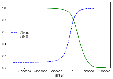
정밀도 곡선이 재현율 곡선보다 굴곡이 있는 이유는,
임계값을 올리더라도 정밀도가 낮아지는 경우가 있기 때문이다.
(상충관계이지만 정밀도가 살짝 줄어들었다가 늘어나는 경우가 있음)
이번에는 정밀도와 재현율 그래프를 그려보자.
plt.plot(recalls[:-1],precisions[:-1])
plt.title("PR곡선")
plt.xlabel("재현율")
plt.ylabel("정밀도")
plt.xlim([0,1])
plt.ylim([0,1])
plt.show()
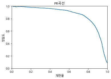
재현율 80% 근처에서 정밀도가 급격히 추락한다. 이 지점의 직전을 트레이드오프로 선택하는 것이 좋다.(재현율 60% 정도)
그리고 이 곡선을 바로 PR곡선 이라고 한다.
3-4. ROC곡선
ROC(Receiver Operating Characteristic)곡선은 정밀도/재현율 곡선과 매우 비슷하지만, 이는 거짓 양성비율(FPR)에 대한 진짜 양성비율(TPR)의 곡선이다.
- 거짓 양성비율(FPR) : 양성으로 잘못 분류된 음성 샘플의 비율
- 진짜 양성비율(TPR) : 재현율
- 진짜 음성비율(TNR) : 1 - FPR => 특이도
from sklearn.metrics import roc_curve
fpr, tpr, thresholds = roc_curve(y_train_5, y_scores)
def plot_roc_curve(fpr, tpr, label=None):
    plt.plot(fpr,tpr, linewidth = 2, label=label)
    plt.plot([0,1],[0,1], 'k--')
    plt.axis([0,1,0,1])
    plt.xlabel('거짓 양성 비율')
    plt.ylabel('진짜 양성 비율')

plot_roc_curve(fpr,tpr)
plt.show()
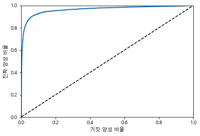
점선은 완전한 랜덤분류기(분류를 하지 않음)의 ROC곡선이며, 좋은 분류기 일수록 점선으로 부터 최대한 멀리 떨어져 있어야 한다.
곡선 아래의 면적을 AUC(Area Under the Curve)라고 하며, 이것으로 분류기들을 비교할 수 있다.
from sklearn.metrics import roc_auc_score
roc_auc_score(y_train_5, y_scores)
0.9636844701880785
랜덤 포레스트 분류기를 훈련시켜 SGDClassifier의 ROC곡선 및 AUC를 비교해보자.
from sklearn.ensemble import RandomForestClassifier

forest_clf = RandomForestClassifier(random_state=42)
y_probas_forest = cross_val_predict(forest_clf, X_train, y_train_5, cv=3,
                                   method="predict_proba")
c:\users\user\appdata\local\programs\python\python37\lib\site-packages\sklearn\ensemble\forest.py:245: FutureWarning: The default value of n_estimators will change from 10 in version 0.20 to 100 in 0.22.
  "10 in version 0.20 to 100 in 0.22.", FutureWarning)
c:\users\user\appdata\local\programs\python\python37\lib\site-packages\sklearn\ensemble\forest.py:245: FutureWarning: The default value of n_estimators will change from 10 in version 0.20 to 100 in 0.22.
  "10 in version 0.20 to 100 in 0.22.", FutureWarning)
c:\users\user\appdata\local\programs\python\python37\lib\site-packages\sklearn\ensemble\forest.py:245: FutureWarning: The default value of n_estimators will change from 10 in version 0.20 to 100 in 0.22.
  "10 in version 0.20 to 100 in 0.22.", FutureWarning)
y_score_forest = y_probas_forest[:,1]
fpr_forest, tpr_forest, thresholds_forest = roc_curve(y_train_5,y_score_forest)
plt.plot(fpr,tpr,"b:",label="SGD")
plot_roc_curve(fpr_forest, tpr_forest, "랜덤포레스트")
plt.legend(loc="lower right")
plt.show()
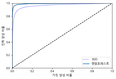
roc_auc_score(y_train_5, y_score_forest)
0.992084014398906
4. 다중분류
지금까지 ‘5맞음’, ‘5아님’을 분류하는 이진분류를 이용했다.
이번에 배울 다중분류기(multiclass classifier)는 둘 이상의 클래스를 구별할 수 있다.
- 이진 분류(서포트 벡터 머신, 선형 분류기 등)
- 다중 분류(랜덤포레스트, 나이브베이즈 등)
- OvA(일대다)전략 : 0부터 9까지(10개의)분류기를 학습시켜 각 분류기의 결정 점수 중 가장 높은 값을 결정
- OvO(일대일)전략 : 0/1, 1/2 등 각 숫자의 조합마다 이진 분류기를 학습
이제 y_tain_5가 아닌 원래 각 숫자마다의 레이블을 가지고 있던 y_train으로 학습해보자.
sgd_clf.fit(X_train, y_train)
c:\users\user\appdata\local\programs\python\python37\lib\site-packages\sklearn\linear_model\stochastic_gradient.py:561: ConvergenceWarning: Maximum number of iteration reached before convergence. Consider increasing max_iter to improve the fit.
  ConvergenceWarning)


SGDClassifier(alpha=0.0001, average=False, class_weight=None,
              early_stopping=False, epsilon=0.1, eta0=0.0, fit_intercept=True,
              l1_ratio=0.15, learning_rate='optimal', loss='hinge', max_iter=5,
              n_iter_no_change=5, n_jobs=None, penalty='l2', power_t=0.5,
              random_state=42, shuffle=True, tol=0.001, validation_fraction=0.1,
              verbose=0, warm_start=False)
sgd_clf.predict([some_digit])
array([5], dtype=int8)
5로 정확히 예측에 성공했다!
some_digit_socres = sgd_clf.decision_function([some_digit])
some_digit_socres
array([[-1.06568587e+05, -4.80037069e+05, -4.83799358e+05,
        -1.59848478e+05, -2.93226642e+05,  4.35583778e+02,
        -6.67998153e+05, -3.90361782e+05, -7.11151233e+05,
        -6.07035899e+05]])
기본적으로 이진분류 알고리즘으로 10개의 분류기를 만들어 학습시키도록 되어 있다.(0임/아님, 1임/아님, …)
따라서 위의 10개의 분류기 점수중 가장 높은 5번째(5)가 가장 점수가 높아 5로 분류했음을 알 수 있다.
np.argmax(some_digit_socres)
5
np.argmax()는 가장 큰 값의 인덱스를 반환한다.
sgd_clf.classes_
array([0, 1, 2, 3, 4, 5, 6, 7, 8, 9], dtype=int8)
classes_속성 클래스의 리스트를 값으로 정렬하여 저장하고 있다.
여기서 OvO나 OvA 전략을 사용하도록 강제하기 위해 OneVsOneClassifier나 OneVsRestClassifier을 사용하면 된다.
from sklearn.multiclass import OneVsOneClassifier

ovo_clf = OneVsOneClassifier(SGDClassifier(max_iter=5, random_state=42))
ovo_clf.fit(X_train, y_train)
ovo_clf.predict([some_digit])
array([5], dtype=int8)
estimators_속성을 이용해 실제로 몇개의 분류기가 사용되었는지 확인할 수 있다.
len(ovo_clf.estimators_)
45
총 10개(0~9)의 숫자를 2개씩 뽑아 조합을 만들었으므로, 10 combination 2 = 45가 맞다.
랜덤포레스트 분류기도 훈련시켜보자.
forest_clf.fit(X_train,y_train)
forest_clf.predict([some_digit])
array([5], dtype=int8)
랜덤포레스트 분류기 자체로 직접 샘플들을 다중분류 하는 것이 가능하기 때문에 OvA나 OvO를 적용할 필요가 없다.
각 클래스별 분류기가 분류한 확률을 확인
forest_clf.predict_proba([some_digit])
array([[0.1, 0. , 0. , 0. , 0. , 0.8, 0. , 0. , 0.1, 0. ]])
다시 SGDClassifier로 돌아와서 교차검증을 시행해보자
cross_val_score(sgd_clf, X_train, y_train, cv = 3, scoring="accuracy")
array([0.86842631, 0.87259363, 0.82372356])
모든 fold에서 80%이상의 정확도를 얻었지만, 스케일링을 통해 성능을 높여보자
from sklearn.preprocessing import StandardScaler

scaler = StandardScaler()
X_train_scaled = scaler.fit_transform(X_train.astype(np.float64))
cross_val_score(sgd_clf, X_train_scaled, y_train, cv = 3, scoring="accuracy")
array([0.90921816, 0.90964548, 0.90973646])
5. 에러분석
이제 모델하나를 결정했다고 가정하고, 성능향상의 방법으로 에러의 종류를 분석해 볼 것이다.
앞에서 만들었던 SGDClassifier로 다시 예측값을 뽑고, confusion matrix를 만들어보자
y_train_pred = cross_val_predict(sgd_clf, X_train_scaled, y_train, cv=3)
conf_mx = confusion_matrix(y_train, y_train_pred)
conf_mx
array([[5741,    3,   18,   10,   10,   43,   42,    8,   44,    4],
       [   1, 6487,   43,   23,    6,   43,    7,   11,  110,   11],
       [  52,   41, 5328,   97,   89,   26,   91,   59,  157,   18],
       [  51,   40,  138, 5336,    3,  227,   38,   52,  144,  102],
       [  22,   27,   32,    8, 5336,   10,   48,   35,   82,  242],
       [  69,   41,   30,  184,   70, 4603,  113,   28,  178,  105],
       [  43,   26,   40,    2,   39,   83, 5628,    8,   48,    1],
       [  24,   18,   70,   31,   54,    8,    4, 5778,   15,  263],
       [  49,  160,   69,  160,   10,  146,   59,   18, 5028,  152],
       [  43,   27,   23,   82,  158,   28,    3,  198,   80, 5307]],
      dtype=int64)
이를 matshow()함수를 이용해 오차행렬을 시각화해보자
plt.matshow(conf_mx, cmap = plt.cm.gray)
plt.show()
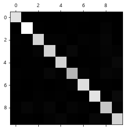
실제로 5가 상대적으로 어두워 보인다.
두가지 이유가 있다.
데이터셋에 5의 이미지가 적거나 / 5를 잘 분류를 못하거나
두가지 모두 확인해 보아야 한다.
각 원소 값을 행별로 열의 값을 모두 더한 값으로 나누어 에러 비율을 비교해보자.
row_sums = conf_mx.sum(axis=1, keepdims=True)
norm_conf_mx = conf_mx / row_sums
np.fill_diagonal(norm_conf_mx, 0)
np.fill_diagonal()함수는 행렬의 대각원소를 입력값으로 대체해 주는 함수이다.
여기서는 대각원소를 0으로 대체했다.(에러비율만 비교하기 위해)
norm_conf_mx
array([[0.        , 0.0005065 , 0.003039  , 0.00168833, 0.00168833,
        0.00725983, 0.007091  , 0.00135067, 0.00742867, 0.00067533],
       [0.00014832, 0.        , 0.00637793, 0.00341145, 0.00088994,
        0.00637793, 0.00103827, 0.00163156, 0.01631563, 0.00163156],
       [0.00872776, 0.0068815 , 0.        , 0.01628063, 0.0149379 ,
        0.00436388, 0.01527358, 0.00990265, 0.02635112, 0.00302115],
       [0.00831838, 0.00652422, 0.02250856, 0.        , 0.00048932,
        0.03702496, 0.00619801, 0.00848149, 0.0234872 , 0.01663676],
       [0.00376583, 0.0046217 , 0.00547758, 0.00136939, 0.        ,
        0.00171174, 0.00821636, 0.0059911 , 0.01403629, 0.04142417],
       [0.01272828, 0.00756318, 0.00553403, 0.03394208, 0.01291275,
        0.        , 0.02084486, 0.0051651 , 0.03283527, 0.01936912],
       [0.00726597, 0.00439338, 0.00675904, 0.00033795, 0.00659006,
        0.01402501, 0.        , 0.00135181, 0.00811085, 0.00016898],
       [0.00383081, 0.0028731 , 0.01117318, 0.00494812, 0.00861931,
        0.00127694, 0.00063847, 0.        , 0.00239425, 0.04197925],
       [0.00837464, 0.02734575, 0.01179286, 0.02734575, 0.00170911,
        0.024953  , 0.01008375, 0.0030764 , 0.        , 0.02597847],
       [0.00722811, 0.00453858, 0.0038662 , 0.01378383, 0.02655909,
        0.00470667, 0.00050429, 0.0332829 , 0.01344764, 0.        ]])
plt.matshow(norm_conf_mx, cmap = plt.cm.gray)
plt.show()
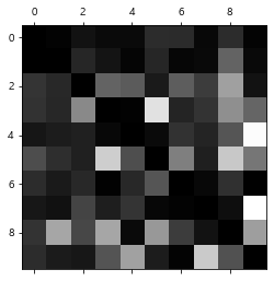
오차행렬(confusion matrix)에서 행은 실제값, 열은 예측값이었다.
- 8과9항목이 상당히 밝게 나타나므로 많은 이미지가 8과9로 잘못 분류되었음을 알 수 있다.(8열 확인)
- 실제값이 8과9인 값들도 다른 값으로 예측된 경우가 많음(8행확인)
- 1은 대부분 정확하게 분류되었고, 일부는 8과 혼돈된 경우가 있음(1열 and 1행 확인)
- 3과 5도 잘 분류를 못하고 있음 (3,5행, 3,5열 확인)
에러가 대칭이 아니라는 점 주의
cl_a, cl_b = 3, 5
X_aa = X_train[(y_train == cl_a) & (y_train_pred == cl_a)]
X_ab = X_train[(y_train == cl_a) & (y_train_pred == cl_b)]
X_ba = X_train[(y_train == cl_b) & (y_train_pred == cl_a)]
X_bb = X_train[(y_train == cl_b) & (y_train_pred == cl_b)]

plt.figure(figsize=(8,8))
plt.subplot(221); plot_digits(X_aa[:25], images_per_row = 5)
plt.subplot(222); plot_digits(X_ab[:25], images_per_row = 5)
plt.subplot(223); plot_digits(X_ba[:25], images_per_row = 5)
plt.subplot(224); plot_digits(X_bb[:25], images_per_row = 5)
plt.show()
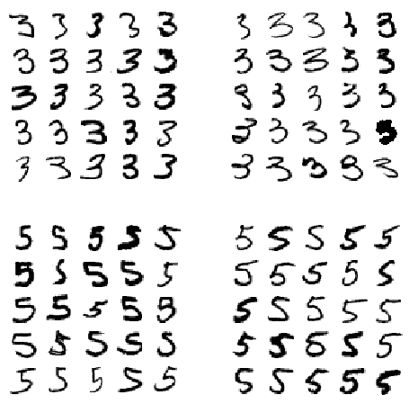
왼쪽 두블록은 분류기가 3으로 예측, 오른쪽 두블록은 5로 예측한 것인데 실제로 봐도 사람도 분류하기 힘들정도로 글씨를 알아보기 어렵다.
이런 경우에 가중치를 주거나, 전처리를 통해 에러를 줄이는 방법을 강구해 볼 필요가 있다.
6. 다중레이블 분류
지금까지는 각 샘플이 하나의 클래스에만 할당(1이면 1, 2면 2)되었다.
하지만 예를들어 사진하나를 주었을때, 사람1, 사람2, 사람3 처럼 사진 하나당 3가지 분류값을 출력해야할 경우가 있다.
이러한 분류시스템을 다중 레이블 분류(Multilabel classification)라고 한다.
y_train_large = (y_train >= 7)
y_train_odd = (y_train % 7 == 1)
y_multilabel = np.c_[y_train_large, y_train_odd]
y_multilabel
array([[False, False],
       [False,  True],
       [ True, False],
       ...,
       [False,  True],
       [ True,  True],
       [ True, False]])
이 두 레이블은 숫자가 큰 값(7이상)인지, 홀수인지를 나타낸다.
이러한 다중 레이블 분류를 지원하는 최근접이웃 분류 알고리즘이 있다.
from sklearn.neighbors import KNeighborsClassifier

knn_clf = KNeighborsClassifier()
knn_clf.fit(X_train, y_multilabel)
KNeighborsClassifier(algorithm='auto', leaf_size=30, metric='minkowski',
                     metric_params=None, n_jobs=None, n_neighbors=5, p=2,
                     weights='uniform')
knn_clf.predict([some_digit])
array([[False, False]])
올바르게 분류되지 않았다..
5는 7보다작고(False), 홀수(True)이므로,
7 다중 출력 분류
다중 출력 분류는 다중 레이블 분류에서 한 레이블이 다중 클래스가 될 수 있도록 일반화 한 것이다.
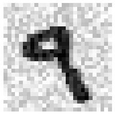
노이즈가 많은 이미지를 입력으로 받아, 깨끗한 숫자 이미지를 MNIST이미지 데이터 처럼 픽셀의 강도를 담은 배열로 출력해보자.
여기서 다중 출력이라는 의미는, 노이즈 제거의 목적으로 한 픽셀당 한 레이블(0~255까지 강도)이기 때문에 각 레이블은 여러개의 값을 가지게 되기 때문이다.
noise = np.random.randint(0, 100, (len(X_train), 784))
X_train_mod = X_train + noise
noise = np.random.randint(0, 100, (len(X_test), 784))
X_test_mod = X_test + noise
y_train_mod = X_train
y_test_mod = X_test

some_index = 36000
some_digit_noise = X_train_mod[some_index]
some_digit_noise_img = some_digit_noise.reshape(28,28)
some_digit = X_train[some_index]
some_digit_img = some_digit.reshape(28,28)
9라는 임의의 숫자를 뽑고, 노이즈를 추가했다.
plt.imshow(some_digit_noise_img, cmap = matplotlib.cm.binary,
          interpolation="nearest")
plt.axis("off")
plt.show()
기존의 x,y가 아니라 둘다 x_train 데이터셋인데 노이즈가 들어있고(독립변수) 안들어있고(종속변수)의 차이이다.
knn_clf.fit(X_train_mod, y_train_mod)
clean_digit = knn_clf.predict([X_train_mod[some_index]])
따라서 predcit의 반환값은, 다중 출력으로 각 픽셀들이 가지는 레이블(강도)로 분류가 된다.
즉, 깨끗한 이미지 픽셀들로 분류기를 학습시켜 노이즈사 섞인 이미지를 깨끗한 이미지중 하나로 분류(깨끗하게 만든다는 의미)하게 만드는 것이다.
plt.imshow(clean_digit.reshape(28,28), cmap = matplotlib.cm.binary,
          interpolation="nearest")
plt.axis("off")
plt.show()

Reference
도서 [Hands-0n Machine Learning with Scikit-Learn & Tensorflow] 를 공부하며 작성하였습니다.

댓글남기기